Manual

Quick Start

To run the examples, just download the data and start the python console. We can then import Fanova and start it by typing

>>> from pyfanova.fanova import Fanova
>>> f = Fanova("example/online_lda")

This creates a new Fanova object and fits the Random Forest on the specified data set. (Note: if you use data generated by SMAC, replace the above path with the path to the state-run directory)

To compute now the marginal of the first parameter type:

>>> f.get_marginal(0)
    5.44551614362

Fanova also allows to specify parameters by their names.

>>> f.get_marginal("Col0")
5.44551614362

If you want to print all marginal at once, you can do that by:

>>> f.print_all_marginals()

But be aware of that may take a while!

Advanced

If you want to take only configurations into account that achieved a better performance than the default configuration you have to set the flag ‘improvement_over=”DEFAULT”’ when you call the Fanova like:

>>> f = Fanova("example/online_lda", improvement_over="DEFAULT")

Furthermore, if you want the Fanova only a certain quantile (let’s say 25%) of the data you can call it by:

>>> f = Fanova("example/online_lda", improvement_over="QUANTILE", quantile_to_compare=0.25)

You can also specify the number of trees in the random forest as well as the minimum number of points to make a new split in a tree by:

>>> f = Fanova("example/online_lda", num_trees=30, split_min=3)

More functions

• Fanova.get_pairwise_marginal(param0, param1)

Returns the pairwise marginals of the two parameter param0 and param1

• Fanova.get_all_pairwise_marginals()

Returns all pairwise marginals

• Fanova.get_most_important_pairwise_marginals(n)

Returns the n most important pairwise marginals

• Fanova.get_marginal_for_value(p, v)

Computes the mean and standard deviation of the parameter p for a certain value v

Visualization

To visualize the single and pairwise marginals, we have to create a visualizer object first

>>> from pyfanova.visualizer import Visualizer
>>> vis = Visualizer(f)

We can then plot single marginals by

>>> plot = vis.plot_marginal("Col1")
>>> plot.show()

what should look like this

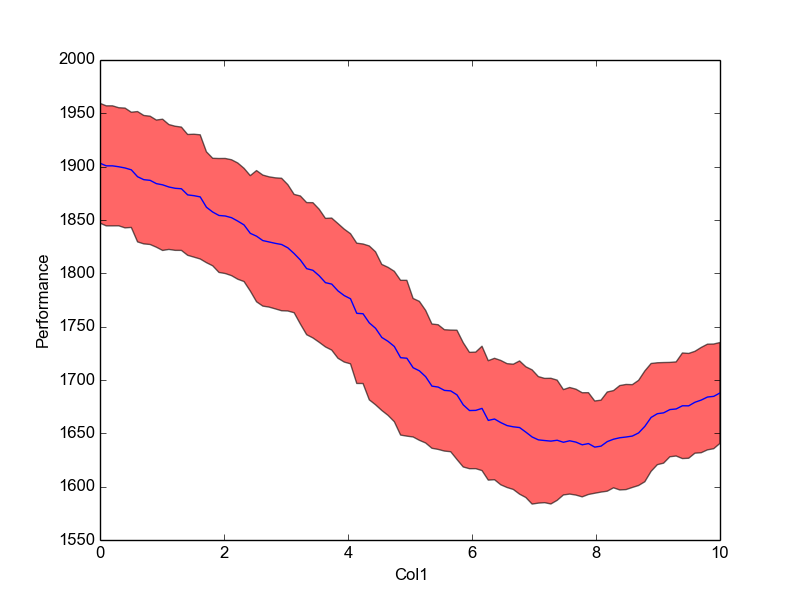
NOTE: For categorical values use the function plot_categorical_marginal() instead.

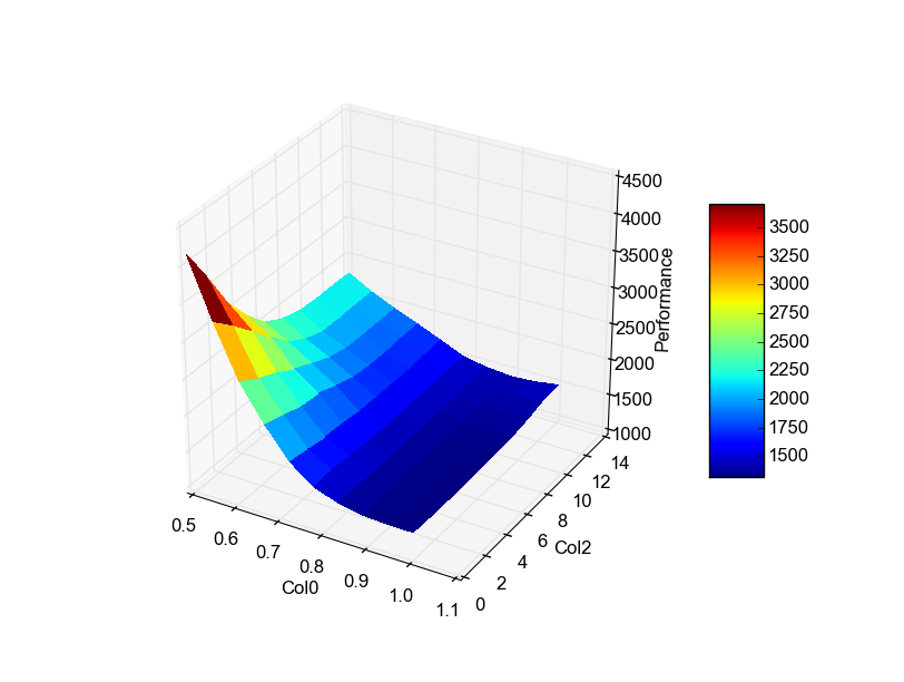
The same can been done for pairwise marginals

>>> vis.plot_pairwise_marginal("Col0", "Col2")

If you are just interested in the N most important pairwise marginals you can plot them through:

>>> create_most_important_pairwise_marginal_plots(dir, N)

and Fanova will save those plot in dir. However, be aware that to create the plots Fanova needs to compute all pairwise marginal, which can take awhile!

At last, all plots can be created together and stored in a directory with

>>> vis.create_all_plots("./plots/")

Start Fanova from CSV-file

If your data is stored in csv file, you can run Fanova with

>>> from pyfanova.fanova_from_csv import FanovaFromCSV
>>> f = FanovaFromCSV("/path_to_data/data.csv")

Please make sure, that your csv file has the form

X0	X1	...	Y
0.1	0.2	...	0.3
0.3	0.4	...	0.6

Start Fanova from HPOlib

It is also possible to run Fanova on data collected by HPOlib

>>> from pyfanova.fanova_from_hpolib import FanovaFromHPOLib
>>> f = FanovaFromHPOLib("params.pcs",["data.pkl"])

Fanova on merged SMAC runs

If you have different SMAC runs from the same task, you can combine them and apply Fanova on the merged data set. This will make the result of Fanova more reliable, simply because it has more data.

To merge different SMAC runs, you have to merge the different state-run order via SMAC’s state-merge tool:

/path_to_smac/util/state-merge --directories /path/state-run* --scenario-file scenario.txt --outdir merged_state_runs/

Afterwards you can start the Fanova with the path to the new state run directory (e.g. “merged_state_runs/”) and it will use the merged data points.